Mmmm…cake
Digital signal processing is a broad and deep topic that is usually covered in a series of engineering courses. But we aren’t going to look at the underlying theory or even take a “cookbook” approach. The theoretical approach looks at the mathematics of DSP, and there many good textbooks and classes at your local colleges to provide this background. These books will provide a rigorous background of z-transforms, sampling theory, bilinear transforms, regions of convergence and other mathematical relationships important for a comprehensive understanding of DSP theory. And there are several good DSP cookbooks that document the equations needed to implement digital filters, transforms and other high-level blocks that provide high-level mathematical solutions without delving as deeply into the theory. If you want to understand the theory or practical applications of the theory, look at the books listed at the end of this article.
We aren’t going to address that level of detail here, in fact, we won’t even get close to that level of detail. Instead, we are going to use what I call a “cake mix”approach, where we have to understand how to open the box, add an egg, and mix the packaged ingredients. The cake won’t be as satisfying as if it were made from scratch, grinding our own flour and understanding the chemical reactions that happen during baking. But in the end we’ll have cake, and that’s important 🙂 .
Key Concepts and Building Blocks
But even with this simplified cake mix approach, we need to understand a few basic DSP terms and operations. We’ll introduce those terms and then move on to the high-level DSP blocks that we will need for designing active speakers.
1. PCM Audio
PCM stands for pulse-code modulation. It is the way analog data is represented in a DSP chip. Analog data is sampled at regular intervals and converted to a numerical value corresponding to the signal amplitude, and those numbers are called pulse-codes. The graphic at Wikipedia article on Pulse-code modulation illustrates the concept of converting analog signals to numeric values:
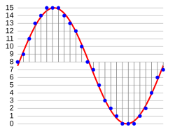
The conversion to PCM is done in the Analog to Digital converter, which is usually referred to as the A/D. And then the codes get converted to audio again in the Digital to Analog, or DAC. The actual codes that are used for each audio–those numbers–are different depending on the type of DSP chip, and that’s a detail we will need to understand to control the volume or other processing. Also, the time between samples is important, but for the designs in this article, the rate will be fixed at 48,000 samples per second, or about 21usec between samples. The PCM data changing at the sampling rate is often referred to as a PCM stream.
Arithmetic Operations
All of the processing inside the DSP chip is done with those digital codes, the PCM data. The DSP will add, multiply and do other operations on those codes using dedicated hardware specific to that chip. Multiplication and addition are done in what is called an Arithmetic Logic Unit (ALU), and some DSP chips may have quite a few ALU’s. The “precision” of the ALU is important for certain operations, and it characterized by the number of bits used to perform the arithmetic operations. See the next article for some details on the amount of precision used by various DSP chips.
Audio routing
Another key concept for DSP chips is audio routing, and the hardware element used for audio routing is called a multiplexer. Audio routing allows control of the flow of the various PCM streams inside the DSP chip. For example, you might have to select between left and right channel PCM streams and route the selected stream to the next processing stage. Audio Routing can also be done with an ALU instead of dedicated multiplexer logic.
Delays
Many DSP chips provide memory dedicated to delaying the PCM stream or individual samples. Delay is implemented by storing samples in memory and then recalling it at a later time. Some of the delays are very short, such as those needed for digital filters. For delays such as needed to compensate for driver alignment or listening position, the delay can be many sample points.
Filters
Just about any DSP chip will provide a way to implement digital filters, and we’ll need a little bit of math to discuss them, but it won’t be much. First is the most commonly used filter, the Infinite Impulse Response (IIR) filter.
The IIR filter uses delays and mixing to provide digital feedback. A very simple IIR filter is shown below, which is from the Wikipedia article on “Infinite impulse response”.

The blocks labeled “Z-1″are one-sample delays that provide feedback from the output. The blocks labeled “SUM” are ALU’s. As new samples arrive, they will get mixed with scaled amounts of the previous output samples, to modify the next output sample. This feedback means that an impulse at the input will continue to show up to some extent in the output forever, depending on how much scaling is used in the “SUM” blocks: hence the term “infinite impulse response”.
A more practical IIR filter uses the structure show below–it is the digital biquad. Again, this picture is taken from the Wikipedia article on IIR.

This biquad structure looks intimidating, but you don’t need to work with this level of detail for active speakers, because we will be able to treat this as a “black box” (or, to use our cake analogy, it’s one of those mysterious chocolate-oid chunks in the cake mix). The blocks labeled “Z-1” are the delays, and the plus symbols are ALU’s. The little triangles represent scale factors that are identified as b0, b1, b2, -a1, and -a2. These scale factors are called the coefficients for the biquad filter. For those who want to see the math, this structure implements a filter that has the following transfer function:

Solving this equation as a function of frequency requires some substitution using complex numbers, and we won’t show those steps here. But once the substitution for those “z” terms is made, this equation can be solved using Excel or any programming language that supports complex numbers.
This transfer function can be used to implement a wide variety of filters. Depending on the value of the coefficients, you can implement any of the following filters:
- Low pass (one or two poles)
- High pass (one or two poles)
- Bandpass
- Notch
- All-Pass
- Peaking
- Shelving (low or high pass)
All we need to do to implement any of these filters is figure out the right coefficient values. It turns out that most of this work has been done for us. Just do a Google search on “Audio-EQ-Cookbook” and you will find the equations needed to design any of these filters. But it’s even simpler than that to use these filters. There are a number of software programs or spreadsheets that solve those equations, and we simply specify the filter parameters (such as the cutoff frequencies, “Q”, and gain) and the program or spreadsheet will calculate the 5 coefficient values we need.
The other type of filter used in DSP chips is the Finite Impulse Response, or FIR filter. These filters are used less often because they require more DSP resources (more memory and more processing cycles to achieve a steep response), but they have some very useful properties for crossovers. The FIR filter structure is shown below (this graphic is a link to the Wikipedia article on Finite Impulse Response):

The design of the FIR filter is similar to the IIR filter, in that there are published sources for the equations needed to calculate the coefficients, and there are software tools that can perform those calculations. However, we’ll save those details for a later case study.
Look-up tables
Another DSP concept we need to mention is look-up tables. Some DSP chips use tables to look up values, and these are especially useful for implementing non-linear functions such as audio compression and dynamic range control. So there might be some DSP processing where you need to fill in table data to get the output you desire for a range of inputs.
Digital Output
A final concept is digital output. Most DSP chips provide a path to output the PCM samples through a serial data stream. The most common format is I2S, which stands for the Inter-IC Sound bus. I2S uses a high speed master clock, a bit clock, a Left/Right clock and a serial data line to connect to other chips.
Cake Mix
The block diagram below is for an older DSP chip (TAS3004), and it shows most of the building blocks we just discussed.

On the left are the audio routing blocks that select between the various inputs. The block diagram doesn’t show the analog to digital converter, but it shows the PCM stream ANALOGIN_L/R that is generated by the A/D. After the routing and summation, the block shows the filters. This chip provides 7 biquad filters for each channel. The Bass/Treble blocks are simply additional biquads configured as shelving filters. The Dynamic Range Control block provides table lookup values to scale the output volume according to the average signal level, and the Saturation Logic does some additional non-linear processing to make sure the digital values do not roll over from positive to negative or vice versa for peak levels.
That block diagram is like a cake mix where all of the low-level details of configuring biquad filters or loudness or routing are done for us: we simply need to add the coefficients, the routing codes and dynamic range thresholds to make this useful for active speakers. Now, it turns out that adding this information will require using a microprocessor and being able to read the data sheets, and that’s going to be a more difficult challenge. But for the most part, the complicated DSP details are hidden from us when we use these chips. We don’t need to understand the math or write DSP code or agonize over z-transforms. We just need to have a basic understanding of the types of DSP processing that takes place inside the chip so we can add our information to the mix.
Fancy Cake Mix
The previous section walked through and older chip design that uses a fixed architecture–that is, there is a fixed number of biquads, multiplexers, ALU’s and a set signal flow through the chip. Newer DSP chips like the ADAU1701 and many TI DSP’s use a reconfigurable architecture, where the computing blocks and signal flow are defined with a graphic user interface. When the user is done defining the processing blocks, the design is “compiled” by a software tool that creates a program for the DSP chip.
Using a programmable architecture provides a lot more flexibility and it allows using some high-level DSP functional blocks and even some complicated algorithms. For example, you can specify a bass enhancement block, or a stereo separation algorithm using the graphical tools, and you simply need to know what parameters to set up to use these block. You don’t need to know the actual processing that takes place–you just need to know what information the processing block requires. Those powerful processing blocks are like having real chocolate chips or toffee bits in the mix!
For an overview of the high-level DSP building blocks available from Analog Devices (the ADAU1701 vendor), follow this link.
Books to read for the mathematical and theoretical details
Obviously, this DSP overview has been trivialized by suggesting that with the right tools, DSP for active speakers can be like making a cake from a mix. Of course, without the right tools it is more like crossing the Sahara on foot, and if you have taken a thorough DSP course at a university, you will probably appreciate that analogy. For those willing to take that trek, the classic textbook is Digital Signal Processing by Oppenheim. For a more practical overview of DSP filters from an implementer’s perspective, take a look at the DSP Filter Cookbook by Lane. Also, there are many good compilations of DSP resources–the one at dspguru.com has a fairly comprehensive list of books and references.